\(2.3.\)序列

1.序列的概念

  序列是一系列有序的值的集合。序列有很多种不同的表示形式，但它们都有以下共同的性质：

• 长度：序列都有有限的长度
• 元素选择。序列的任意元素有一个小于其长度的索引元素，对于第一个元素从\(0\)开始。

二、序列基础

1.\(Lists\)的概念及操作

  \(list\)是一个可以具有任意长度的序列。\(list\)具有大量的内置行为，以及表示这些行为的特定语法。如下是几个\(list\)的例子：

digits=[1,8,2,8]
>>> len(digits)
4
>>> digits[3]
8

  初始化\(list\)、构造一个空\(list\)的步骤如下：

result = [[] for i in player_indices]#初始化为空列表
result = [[0 for m in range(len(n)-1)] for n in times_per_player]#初始化为0

  对于\(list\)，加法和乘法与数学运算中不同，而是组合和复制序列本身。也就是说，运算符模块(和+运算符)中的add函数生成一个列表，该列表是所添加参数的串联。运算符中的mul函数(以及*运算符)可以获取一个列表和一个整数\(k\)，以返回由原始列表的\(k\)重复组成的列表。

>>> [2,7] + digits * 2
[2,7,1,8,2,8,1,8,2,8]

  同时，也可以在\(list\)中嵌套\(list\)，嵌套与访问的方式如下：

pairs=[[10,20],[30,40]]
>>> pairs[1]
[30,40]
>>> pairs[1][0]
30

2.序列迭代

  在许多情况下，我们希望对序列的元素进行迭代，并依次为每个元素执行一些计算。

  \(a.\)\(for\)语句

  \(for\)语句的声明如下：

for <name> in <expression>:
    <suite>

  \(for\)语句的执行过程如下：

1. 计算\(expression\)，\(expression\)必须产生一个可迭代的值。

2. 对于可迭代值的每一个元素值执行：

   1. 将<name>绑定到当前框架中的值。
   2. 执行<suite>。

  \(b.\)\(range\)语句

  \(range\)的声明如下：

range(1,10) # Includes 1, but not 10

  在\(list\)中调用\(range\)可返回\(range\)范围内的\(list\)：

>>> list(range(5,8))
[5,6,7]

  如果\(range\)函数只传了一个参数，那么就返回从\(0\)到\(i-1\)间的序列：

>>> list(range(4))
[0, 1, 2, 3]

  \(range\)经常与\(for\)结合，以达到迭代\(list\)的一部分的目的。这里有一种特殊情况：当<name>='_'时，整个序列会被重复\(i\)次：

>>> for _ in range(3):
        print('Go Bears!')

Go Bears!
Go Bears!
Go Bears!

  \(c.\)序列解包

  当某个\(list\)的内部仍然为\(list\)，但内部的\(list\)长度固定时，我们可以在调用\(for\)循环时使用多个<name>，以打开内部的\(list\)，读取其中元素。下举一例：

>>> pairs=[[1,2],[2,2],[2,3],[4,4]]

for x,y in pairs:
    if(x==y):
        same_count+=1

>>> same_count
2

  这一操作与我们在将多个名称绑定到多个值的赋值语句中看到的模式相同。

三、对序列的基本处理

1.列表解析\(List\;Comprehension\)

  有时我们要对序列中的所有元素执行一个统一的操作，并输出处理后的序列。这时我们可以用列表解析的方法：

#改变列表元素的值
>>> odds=[1,3,5,7,9]
>>> [x+1 for x in odds]
[2,4,6,8,10]

#将列表元素归到其他结构里面
>>>s=[1, 2, 3]
>>>t=[4, 5, 6]
[[s[i]+t[i]]for i in range(len(s))]
>>>[[1, 4], [2, 5], [3, 6]]

  这里的\(for\)并不是\(for\)语句的一部分，而是列表解析的一部分。

  同时，我们也可以只解析序列符合要求的部分，即原序列的子集，下举一例：

>>> [x for x in odds if 25 % x == 0]
[1,5]

  列表解析的一般形式为：

[<map expression> for <name> in <sequence expression> if <filter expression>]

  当要表达不同分支时，可如下书写列表解析：

[<map expression> if <expression> else <map expression> for <name> in <seq>]

2.数据合并

  数据合并，顾名思义，就是将序列中的所有数据最终合并成一个数据。常见的\(min\)、\(max\)、\(sum\)函数都属于数据合并。

3.利用高阶函数抽象序列基本操作

  上述序列操作可通过高阶函数、以函数为参数的手段来抽象出更普适的模式：

• 对序列全体元素的映射：

  def apply_to_all(map_f,s):
      return [map_f(i) for i in s]

• 筛选元素：

  def keep_if(filter_f,s):
      return [i for i in s if filter_f(i)]

• 数据合并：

  def reduce(reduce_f,s,init):
      reduced=init
      for i in s:
          reduced=reduce_f(reduced,i)
      return reduced

4.序列基本处理的应用

  通过使用上述序列基本处理手段，我们可以利用序列处理很多问题。

  \(e.g.\)求出\(1\sim 1000\)内的所有完全数。

  \(solve\)：先利用列表解析写出求某个数因数的函数：

def div(n):
    return [1]+[i for i in range(2,n) if n%i==0]
>>> divisors(12)
[1, 2, 3, 4, 6]

  求出所有因数后，我们将所有因数合并为\(sum\)，继续利用列表解析筛选：

def perfect(n):
    return [1]+[i for i in range(1,1000) if sum(div(i))==i]
>>>[6, 28, 496]

  同时我们的\(div\)函数可以复用以解决以下问题：

  \(e.g.\)给定矩形面积，求矩形的最小周长。

  \(solve\)：矩形的边长只可能是\(div(area)\)中的某个数，于是可写出如下程序：

def width(area,hei):
    assert area%hei==0
    return area//hei

def perimeter(hei,width):
    return 2*hei+2*width

def min_per(area):
    hei=div(area):
    per=[perimeter(h,width(area,h)) for h in hei]
    return min(per)

>>> area=80
>>> width(area,5)
16
>>> perimeter(10, 8)
36
>>> min_per(area)
36
>>> [minimum_perimeter(n) for n in range(1, 10)]
[4, 6, 8, 8, 12, 10, 16, 12, 12]

  这些操作并不是一定需要序列来实现，但是序列上述基本操作的存在极大地降低了实现的难度。将问题序列化不失为一种解题策略。

四、序列抽象

  序列抽象分为以下部分(前两点前文已提及)：

1.序列长度

>>> digits = [1, 8, 2, 8]
>>> len(digits)
4

2.序列选择

>>> digits[3]
8

3.判断是否为序列成员

>>> digits
[1, 8, 2, 8]
>>> 2 in digits
True
>>> 1828 not in digits
True

4.剪切序列片段

>>> digits[0:2]
[1, 8]
>>> digits[1:]
[8, 2, 8]

五、\(string\)

六、\(Trees\)

1.引入——闭包性质

  在\(list\)中，我们可以使用\(list\)作为\(list\)的元素，这种数据的组合方式被称为数据的闭包性质。

  在任何组合方式中，闭包性质都是组合的关键，因为它允许我们创造一种组合方式的等级结构——一种组合由与它相同的子组合构成，而子组合又由更小的子组合构成...如下即为\(list\)的等级结构示意图：

one_two = [1, 2]
    nested = [[1, 2], [],
    [[3, False, None],
    [4, lambda: 5]]]

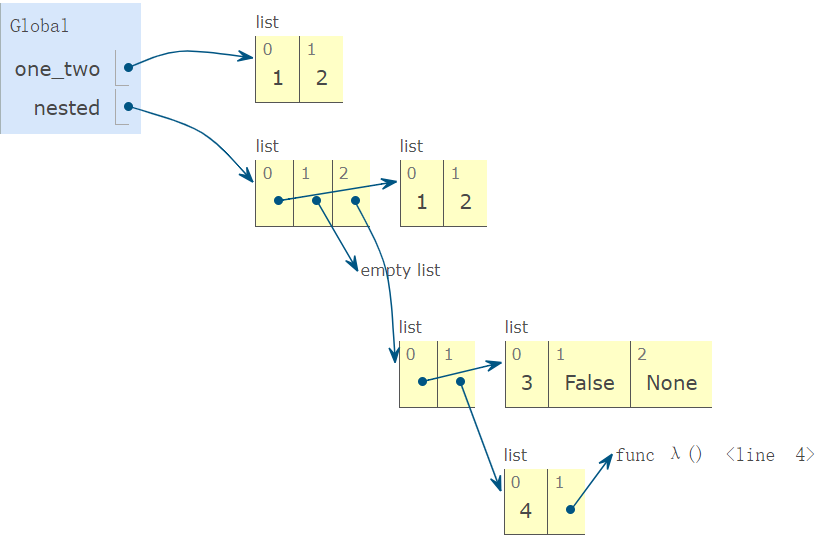
  这种嵌套结构会引入复杂性，让我们能更好地处理复杂的数据。\(Trees\)和之后的数据结构都是这样的嵌套结构

2.树的概念

  树是由树根与树枝序列组成的。树的每根树枝也是一棵树。没有树枝的节点被称为叶子结点。每棵树的树根被称作根节点。

3.树的代码实现

  \(a.\)树的相关概念的实现

  树这种数据抽象形式的实现由\(constructor\)tree与\(selector\)branches，root构成：

def tree(root_label,branches=[]):#将branches强制转化为list结构
    for branch in branches:
        assert is_tree(branch),'branches must be trees'
    return [root_label]+list(branches)

def label(tree):
    return tree[0]

def branches(tree):
    return tree[1:]

def is_tree(tree):
    if(type(tree)!=list or len(tree)<1):
        return False
    for branch in branches(tree):
        if not is_tree(branch):
            return False
    return True

def is_leaf(tree):
    return not branches(tree)

  树可以由嵌套表达式构造，如下所示：

>>> t = tree(3, [tree(1), tree(2, [tree(1), tree(1)])])
>>> t
[3, [1], [2, [1], [1]]]
>>> label(t)
3
>>> branches(t)
[[1], [2, [1], [1]]]
>>> label(branches(t)[1])
2
>>> is_leaf(t)
False
>>> is_leaf(branches(t)[0])
True

  \(b.\)树形递归的使用

  由于树本身的层次性，利用树形递归也可得出树的一些性质。

def count_leaves(tree):
    if is_leaf(tree):
        return 1
    else:
        branches_count=[count_leaves(b) for b in branches(tree)]
        return sum(branch_counts)

  可以发现我们对树结构的处理是在\(list\)的层面上处理，当我们需要读取具体的结果时才利用数据合并的操作\(return\)一个整数。

  \(c.\)限制树的树枝数

  为限制树的树枝数，以构建二叉树为例，当树枝长度超过\(2\)时，我们就将树的第一个元素保持不变，而将其余元素作为右分支的子树。即可：

def right_binarize(tree):
    if is_leaf(tree):
        return tree
    if len(tree)>2:
        tree=[tree[0],tree[1:]]
    return [right_binarize(b) for b in tree]

  注意该函数的目标是对整棵树进行右分支重建，因此是for b in tree。

  \(d.\)树的列表化处理

  当我们要对树的某一层节点执行一些操作时，可以考虑如下思路：

1. 将所有节点装进一个\(list\)中
2. 利用序列操作对\(list\)进行处理
3. 将\(list\)回带到树上

  这种将一种序列类型转化为其他类型的序列从而简化操作的方法值得学习。

  \(e.g.\)Write a function reverse_other that mutates the tree such that labels on every other (odd-depth) level are reversed. For example, Tree(1,[Tree(2, [Tree(4)]), Tree(3)]) becomes Tree(1,[Tree(3, [Tree(4)]), Tree(2)]). Notice that the nodes themselves are not reversed; only the labels are.

def reverse_other(t):
    def helper(t,index):
        if not t.is_leaf():
            if index%2==0:
                treelist=[]
                for b in t.branches:
                    treelist.append(b.label)
                treelist.reverse()
                for i in range(len(t.branches)):
                    t.branches[i].label=treelist[i]

            for b in t.branches:
                helper(b,index+1)

    helper(t,0)

3.树的应用

  利用树形递归求解的问题都可以转化到树结构上。以之前的\(Fib\)数列和数的分解为例：

  \(a.\)\(Fib\)数列

  \(Fib\)数列的树结构搭建如下：

def fib_tree(n):
    if(n==0 or n==1):
        return 1
    else:
        left,right=fib_tree(n-1),fib_tree(n-2)
        fib_n=label(left)+label(right)#根节点为左右根节点的和
        return tree(fib_n,[left,right])

>>> fib_tree(5)
[5, [2, [1], [1, [0], [1]]], [3, [1, [0], [1]], [2, [1], [1, [0], [1]]]]]

  这样，每棵树的根节点就表示对应的\(Fib\)数列的值了。

  \(b.\)分解树

  在先前的分解数字中，我们将数字分解分为两种情况：

• 选一个\(m\)，然后对\(n-m\)执行相同操作
• 不选\(m\)，此时序列中最大值变为\(m-1\)，然后继续执行相同操作

  这两种情况分别对应根节点的两个树枝：

• 左树枝：所有至少用一个\(m\)的分解\(n\)的方法
• 右树枝：最大为\(m-1\)的分解\(n\)的方法
• 根节点：\(m\)

  于是可以写出对应的树的构建：

def partition_tree(n,m):
    if n==0:
        return tree(True)
    elif n<0 or m<1:
        return tree(False)
    else:
        left=partition_tree(n-m,m)
        right=partition_tree(n,m-1)
        return tree(m,[left,right])
    
>>> partition_tree(2, 2)
[2, [True], [1, [1, [True], [False]], [False]]]

  若要打印该树，可以将树的根节点转化为\(string\)类型，然后递归打印：

def print_parts(tree,partition=[]):
    if is_leaf(tree):
        if label(tree):#如果不是空节点
            print('+'.join(partition))
    else:
        left,right=branches(tree)//序列解包
        m=str(label(tree))
        print_parts(left,partition+m)
        print_parts(right,partition+m)

>>> print_parts(partition_tree(6, 4))
4 + 2
4 + 1 + 1
3 + 3
3 + 2 + 1
3 + 1 + 1 + 1
2 + 2 + 2
2 + 2 + 1 + 1
2 + 1 + 1 + 1 + 1
1 + 1 + 1 + 1 + 1 + 1

七、\(Linked\;lists\)

1.链表的概念

  如下所示的序列结构就是链表：

four = [1, [2, [3, [4, 'empty']]]]

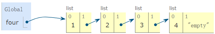
  链表表示若干个\(pair\)，第一个\(pair\)包括第一个元素和一个子链表，以此类推；最后一个\(pair\)包含最后一个元素和空链表empty。可以看出链表具有递归的结构。

2.链表的操作

  \(a.\)链表的基本元素

def first(s):
    return s[0]

def rest(s):
    return s[1]

  \(b.\)链表的长度与元素访问

  作为序列的一种形式，序列抽象的操作在链表中亦可实现：

def len_link(s):
    length=0
    while s!=empty:
        s,length=rest(s),length+1
    return length

def getitem_link(s,i):
    while i>0:
        s,i=rest(s),i-1
    return first(s)

>>> len_link(four)
4
>>> getitem_link(four, 1)
2

  \(c.\)链表的“序列基本操作”

def extend_link(s,t):
    #Return a list with the elements of s followed by those of t.
    assert is_link(s) and is_link(t)
    if s==empty:
        return t
    else:
        return link(first(s),extend_link(rest(s),t))

>>> extend_link(four, four)
[1, [2, [3, [4, [1, [2, [3, [4, 'empty']]]]]]]]

def apply_to_all_link(f,s):
    assert is_link(s)
    if s==empty:
        return s
    else:
        return link(f(first(s)),apply_to_all_link(f,rest(s)))

>>> apply_to_all_link(lambda x: x*x, four)
[1, [4, [9, [16, 'empty']]]]

def keep_if_link(f,s):
    #Return a list with elements of s for which f(e) is true.
    assert is_link(s)
    if s==empty:
        return s
    else:
        kept=keep_if_link(f,rest(s))
        if f(first(s)):
            return link(first(s)+kept)
        else:
            return kept

>>> keep_if_link(lambda x: x%2 == 0, four)
[2, [4, 'empty']]

def join_link(s,separator):
    #Return a string of all elements in s separated by separator.
    if s==empty:
        return ""
    elif rest(s)==empty:
        return str(first(s))
    else:
        return str(first(s))+separator+join_link(rest(s),separator)
    
>>> join_link(four, ", ")
'1, 2, 3, 4'

3.链表的应用

  链表在递增构造序列方面非常有用，因为链表允许动态添加元素、而不必一开始知道序列全部内容

  以先前的数的分解为例，可以用列表如下实现：

def partition(n,m):
    if n==0:
        return link(empty,empty)
    elif n<0 or m<1:
        return empty
    else:
        using_m=partition(n-m,m)
        with_m = apply_to_all_link(lambda s: link(m, s), using_m)
        # creat a list that starts with m
        without_m = partitions(n, m-1)
        return extend_link(with_m, without_m)