8.4.摊还分析

发表于 2024-05-31 更新于 2024-06-02 分类于 CS61B DataStructure ， 8.Effecient Programming 阅读次数：本文字数： 838 阅读时长 ≈ 3 分钟

\(8.4\)摊还分析

与\(O\)相同，\(\Omega\)描述的也是不等关系：如果对于任一比\(N_0\)大的\(N\)，存在\(k_1\)使得\(R(N)\geq k_1·f(N)\)，有：\(R(n)\in \Omega(f(n))\)。

关于\(\Omega\)有以下两个结论：

\(R(n)=O(f(n)),R(n)=\Omega(f(n))\Rightarrow R(n)=\Theta(f(n))\)。
它用于分析算法的基本复杂度。例如，对于重复查找问题(\(duplicate-finding\))，有\(R(n)=\Omega(n)\)，这说明该问题的时间复杂度最小不得超过\(n\)(因为每个元素至少要遍历一次)。

考虑下面的问题：

\(e.g.\)There are two choices to feed Grigometh:

Choice 1: Every day, Grigometh eats 3 bushels of hay from your urn.
Choice 2:Grigometh eats exponentially more hay over time, but comes exponentially less frequently. Specifically:
- On day 1, he eats 1 bushel of hay (total 1)
- On day 2, he eats 2 additional bushels of hay (total 3)
- On day 4, he eats 4 additional bushels of hay (total 7)
- On day 8, he eats 8 additional bushels of hay (total 15)

选择\(1\)每次只用放置常数个干草，然而事实上，选择\(2\)需要的干草数量更少，因为：

这里我们采用的方法是将所有天数干草的总和“均摊”到每一天。可以看到，选择\(2\)的每日干草消耗量实际上是常数。我们将选择\(2\)的情况称为均摊常数。

更为严谨的摊还分析流程如下：

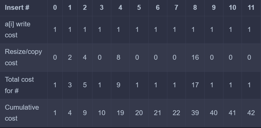
以我们的数组扩容为例，对于数组扩容，我们每次需要执行的操作如下：

x.add(0) performs 1 write operation. No resizing. Total: 1 operation
x.add(1) resizes and copies the existing array (1 read, 1 write), and then writes the new element. Total: 3 operations
x.add(2) resizes and copies the existing array (2 reads, 2 writes), and then writes the new element. Total: 5 operations
x.add(3) does not resize, and only writes the new element. Total: 1 operations
x.add(4) resizes and copies the existing array (4 reads, 4 writes), and then writes the new element. Total: 9 operations

我们可以列出如下的表格：

我们接着引入“势能”(\(potential\))的概念。对于每个操作\(i\)，令\(c_i\)为该操作的真实时间耗费，令\(a_i\)为任一摊还时间消耗。对于常数时间消耗，\(a_i\)也必须是常数。

我们令\(\Phi_i\)为操作\(i\)的势能，用于表示摊还消耗和真实消耗间的累积差距(\(difference\))，则：\(\Phi_i=\Phi_{i-1}+a_i-c_i\)。

\(a_i\)可以是任一我们选择的数。如果对于我们选择的\(a_i\)，\(\Phi_i\)永远是非负的，那么我们预测的摊还消耗就是实际消耗的上界。如果\(a_i\)为一个永远不变的常数，那么实际消耗就是以常数时间为上界，这即说明该函数的平均时间消耗为常数！

对于数组扩容，可以列出以下表格：

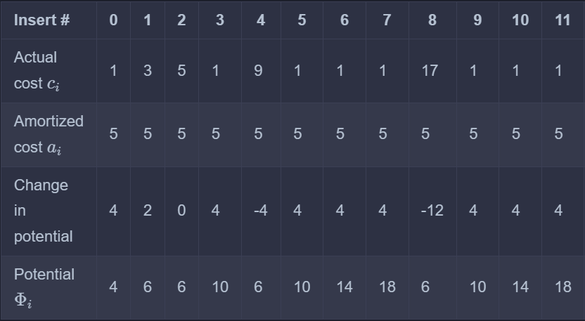
可以看出，势能一直是非负的。这样，我们就可以宣称：数组扩容的操作的摊还时间是常数。