\(4.4.\)General Principles of Pipelining

1.Computational Pipelines

  The detail at the timing and operation of this process are shown as below:

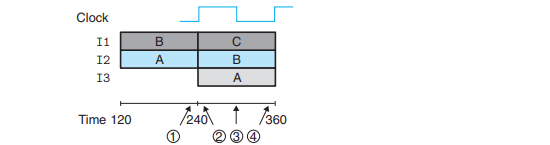
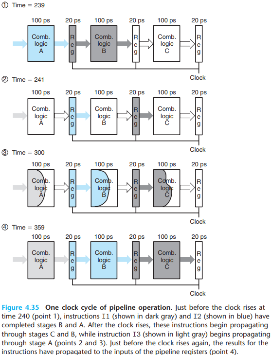
• Slowing down the clock would not change the pipeline behavior. The signals propagate to the pipeline register inputs, but no change in the register states will occur until the clock rises.

2.Limitations of Pipelining

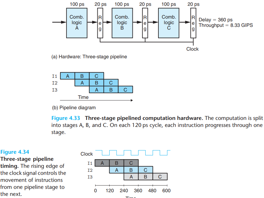
  \(a.\)Throughput

  Suppose the maximum delay of a process is \(x\) ps, then we can calculate the throughput as:

\[ throughput={ {1\;instruction}\over{x\;ps} } \cdot { {1000\;ps} \over {1\;ns}}={1000\over x}GIPS \]

  And the latency is the overall time the process takes.

  \(b.\)Nonuniform partition

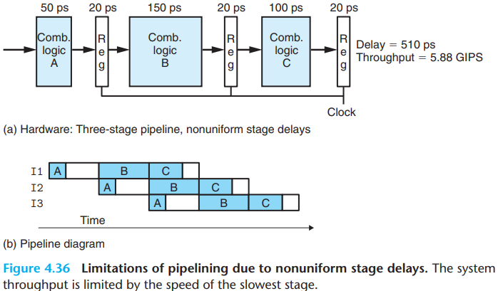
• The latency of piplining is decided by the slowest clock rate.

  • For the process above, delays of A and C are 50ps and 100+20 = 120 ps, while delay of B is 150+20 = 170ps, so we have to set the clock cycle to 170ps.

Note that the delay of pipeline register is included in register that fetch data from it. So in the process above, B and C should add the 20ps delay.

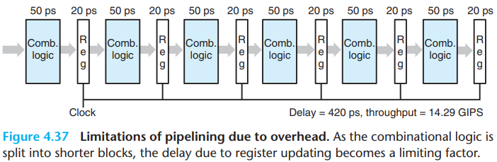
  \(c.\)Diminishing returns of deep pipelining

3.Piplining a System with Feedback

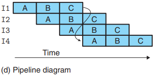
  For a system that executes machine programs such as Y86-64, there are potential dependencies between successive instructions.

• The following codes describe what is called data dependency. The irmovq instruction stores its result in %rax, which then must be read by the addq instruction.

irmovq $50, %rax
addq %rax, %rbx
mrmovq 100(%rbx), %rdx

• The following codes describe what is called control dependency. The outcome of the conditional test determines whether the next instruction to execute:

loop:
    subq %rdx,%rbx
    jne targ
    irmovq $10,%rdx
    jmp loop
targ:
    halt